Chapter 7 Matching
Having learned about matching techniques, you may wonder whether you could use them to estimate the impact of the Health Insurance Subsidy Program (HISP). You decide to use some matching techniques to select a group of nonenrolled households that look similar to the enrolled households based on baseline observed characteristics.
To do so, you will conduct Propensity Score Matching (PSM). The Propensity Score is the probability that a household will enroll in the program based on the observed values of characteristics (the explanatory variables), such as the age of the household head and of the spouse, their level of education, whether the head of the household is a female, whether the household is indigenous, and so on.
Before we start we need to put the data in wide format. Currently a household covers multiple rows in our dataset, as variables are measured pre- and post-enrollment. As we want to match households, we instead each row to be a unique household. Therefore, we have to widen the dataset, by creating separate columns for household characteristics in each time period.
df_w <- df %>%
  pivot_wider(names_from = round, # variable that determines new columns
              # variables that should be made "wide"
              values_from = c(health_expenditures,
                              poverty_index, age_hh, age_sp,
                              educ_hh, educ_sp, female_hh,
                              indigenous, hhsize, dirtfloor,
                              bathroom, land, hospital_distance,
                              hospital)) %>%
  # remove the household that has missing values
  # as missing values are not allowed when using matchit
  filter(!is.na(health_expenditures_0))
We will carry out matching using two scenarios. In the first scenario, there is a large set of variables to predict enrollment, including socioeconomic household characteristics. In the second scenario, there is little information to predict enrollment (only education and age of the household head).
Estimate the Propensity Score
# We'll conduct propensity score estimation and matching at the same
# time, as the matchit function does this for us
psm_r <- matchit(enrolled ~ age_hh_0 + educ_hh_0,
                 data = df_w %>% dplyr::select(-hospital_0, -hospital_1),
                 distance = "probit")
psm_ur <- matchit(enrolled ~ age_hh_0 + educ_hh_0 + age_sp_0 + educ_sp_0 +
                    female_hh_0 + indigenous_0 + hhsize_0 + dirtfloor_0 +
                    bathroom_0 + land_0 + hospital_distance_0,
                 data = df_w %>% dplyr::select(-hospital_0, -hospital_1),
distance = "probit")htmlreg(list(psm_r$model, psm_ur$model),
doctype = FALSE,
custom.coef.map = list('age_hh_0' = "Age (HH) at Baseline",
'educ_hh_0' = "Education (HH) at Baseline",
'age_sp_0' = "Age (Spouse) at Baseline",
'educ_sp_0' = "Education (Spouse) at Baseline",
'female_hh_0' = "Female Head of Household (HH) at Baseline",
'indigenous_0' = "Indigenous Language Spoken at Baseline",
'hhsize_0' = "Number of Household Members at Baseline",
'dirtfloor_0' = "Dirt floor at Baseline",
'bathroom_0' = "Private Bathroom at Baseline",
'land_0' = "Hectares of Land at Baseline",
'hospital_distance_0' = "Distance From Hospital at Baseline"),
caption = "Estimating the Propensity Score Based on Baseline Observed Characteristics",
custom.model.names = c("Limited Set", "Full Set"))| Limited Set | Full Set | |
|---|---|---|
| Age (HH) at Baseline | -0.02*** | -0.01*** |
| (0.00) | (0.00) | |
| Education (HH) at Baseline | -0.04*** | -0.02*** |
| (0.01) | (0.01) | |
| Age (Spouse) at Baseline | -0.01*** | |
| (0.00) | ||
| Education (Spouse) at Baseline | -0.02* | |
| (0.01) | ||
| Female Head of Household (HH) at Baseline | -0.02 | |
| (0.05) | ||
| Indigenous Language Spoken at Baseline | 0.16*** | |
| (0.03) | ||
| Number of Household Members at Baseline | 0.12*** | |
| (0.01) | ||
| Dirt floor at Baseline | 0.38*** | |
| (0.03) | ||
| Private Bathroom at Baseline | -0.12*** | |
| (0.03) | ||
| Hectares of Land at Baseline | -0.03*** | |
| (0.01) | ||
| Distance From Hospital at Baseline | 0.00*** | |
| (0.00) | ||
| AIC | 11658.35 | 11037.04 |
| BIC | 11679.96 | 11123.46 |
| Log Likelihood | -5826.18 | -5506.52 |
| Deviance | 11652.35 | 11013.04 |
| Num. obs. | 9913 | 9913 |
| p < 0.001; p < 0.01; p < 0.05 | ||
As shown in the above table, the likelihood that a household is enrolled in the program is smaller if the household is older, more educated, headed by a female, has a bathroom, or owns larger amounts of land. By contrast, being indigenous, having more household members, having a dirt floor, and being located further from a hospital all increase the likelihood that a household is enrolled in the program. So overall, it seems that poorer and less-educated households are more likely to be enrolled, which is good news for a program that targets poor people.
Plot the distribution of the Propensity Score by enrollment. What can we say about common support?
df_w <- df_w %>%
  mutate(ps_ur = psm_ur$model$fitted.values)

df_w %>%
  mutate(enrolled_lab = ifelse(enrolled == 1, "Enrolled", "Not Enrolled")) %>%
  ggplot(aes(x = ps_ur,
             group = enrolled_lab, colour = enrolled_lab, fill = enrolled_lab)) +
  geom_density(alpha = I(0.2)) +
  xlab("Propensity Score") +
  scale_fill_viridis_d("Status:", end = 0.7) +
  scale_colour_viridis_d("Status:", end = 0.7) +
  theme(legend.position = "bottom")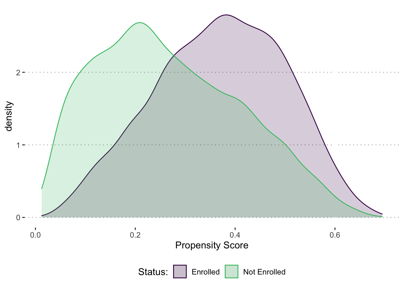
Figure 7.1: Distribution of Propensity Score by Enrollment Status
You check the distribution of the propensity score for the enrolled and matched comparison households. Figure 7.1 shows that common support (when using the full set of explanatory variables) extends across the whole distribution of the propensity score. In fact, none of the enrolled households fall outside the area of common support. In other words, we are able to find a matched comparison household for each of the enrolled households.
Did matching by the propensity score improve balance?
| Means Treated | Means Control | SD Control | Mean Diff | eQQ Med | eQQ Mean | eQQ Max | |
|---|---|---|---|---|---|---|---|
| distance | 0.3694119 | 0.2683525 | 0.1435197 | 0.1010594 | 0.1109167 | 0.1010943 | 0.1284425 |
| age_hh_0 | 41.6565796 | 48.1384372 | 15.5146171 | -6.4818576 | 7.0000000 | 6.4925432 | 10.0000000 |
| educ_hh_0 | 2.9711803 | 2.7744736 | 2.7971992 | 0.1967067 | 0.0000000 | 0.3312010 | 4.0000000 |
| age_sp_0 | 36.8363698 | 41.6117427 | 12.9925496 | -4.7753729 | 5.0000000 | 4.7908232 | 9.0000000 |
| educ_sp_0 | 2.7032726 | 2.5810189 | 2.5713309 | 0.1222538 | 0.0000000 | 0.2663630 | 4.0000000 |
| female_hh_0 | 0.0732119 | 0.1100878 | 0.3130217 | -0.0368759 | 0.0000000 | 0.0367746 | 1.0000000 |
| indigenous_0 | 0.4291498 | 0.3203339 | 0.4666384 | 0.1088159 | 0.0000000 | 0.1089744 | 1.0000000 |
| hhsize_0 | 5.7699055 | 4.9263203 | 2.2276936 | 0.8435852 | 1.0000000 | 0.8468286 | 2.0000000 |
| dirtfloor_0 | 0.7216599 | 0.5533170 | 0.4971849 | 0.1683429 | 0.0000000 | 0.1683536 | 1.0000000 |
| bathroom_0 | 0.5735493 | 0.6340481 | 0.4817307 | -0.0604988 | 0.0000000 | 0.0603914 | 1.0000000 |
| land_0 | 1.6771255 | 2.2511153 | 3.3057321 | -0.5739898 | 0.0000000 | 0.5779352 | 5.0000000 |
| hospital_distance_0 | 109.2043122 | 103.6626222 | 42.0414242 | 5.5416899 | 5.2651255 | 5.7016559 | 13.5770481 |
| Means Treated | Means Control | SD Control | Mean Diff | eQQ Med | eQQ Mean | eQQ Max | |
|---|---|---|---|---|---|---|---|
| distance | 0.3694119 | 0.3687162 | 0.1289918 | 0.0006957 | 0.0001013 | 0.0007221 | 0.0167152 |
| age_hh_0 | 41.6565796 | 41.7867746 | 13.1422452 | -0.1301951 | 1.0000000 | 0.8650129 | 5.0000000 |
| educ_hh_0 | 2.9711803 | 2.9549320 | 2.7497469 | 0.0162484 | 0.0000000 | 0.1437787 | 4.0000000 |
| age_sp_0 | 36.8363698 | 36.9915655 | 11.0374258 | -0.1551957 | 1.0000000 | 0.7699055 | 8.0000000 |
| educ_sp_0 | 2.7032726 | 2.7128880 | 2.6196748 | -0.0096154 | 0.0000000 | 0.1378205 | 4.0000000 |
| female_hh_0 | 0.0732119 | 0.0732119 | 0.2605279 | 0.0000000 | 0.0000000 | 0.0000000 | 0.0000000 |
| indigenous_0 | 0.4291498 | 0.4234143 | 0.4941832 | 0.0057355 | 0.0000000 | 0.0057355 | 1.0000000 |
| hhsize_0 | 5.7699055 | 5.7884615 | 2.1411833 | -0.0185560 | 0.0000000 | 0.1373144 | 1.0000000 |
| dirtfloor_0 | 0.7216599 | 0.7253711 | 0.4464024 | -0.0037112 | 0.0000000 | 0.0037112 | 1.0000000 |
| bathroom_0 | 0.5735493 | 0.5732119 | 0.4946944 | 0.0003374 | 0.0000000 | 0.0003374 | 1.0000000 |
| land_0 | 1.6771255 | 1.7010796 | 2.6217989 | -0.0239541 | 0.0000000 | 0.1103239 | 3.0000000 |
| hospital_distance_0 | 109.2043122 | 108.5100383 | 41.8790212 | 0.6942738 | 1.2450775 | 1.6190618 | 7.5290520 |
Using the matched sample, what is the estimated effect of the program?
To obtain the estimated impact using the matching method, we first need to extract the matched data set.
We can then estimate the effect of the program using a (weighted) linear regression. In this case all weights are equal to 1, meaning there is no need to use the weights, as we have one to one matching without replacement.
out_lm_r <- lm_robust(health_expenditures_1 ~ enrolled,
                      data = match_df_r, clusters = locality_identifier,
                      weights = weights)
out_lm_ur <- lm_robust(health_expenditures_1 ~ enrolled,
                      data = match_df_ur, clusters = locality_identifier,
weights = weights)htmlreg(list(out_lm_r, out_lm_ur),
doctype = FALSE,
caption = "Evaluating HISP: Matching on Baseline Characteristics and Regression Analysis",
custom.model.names = c("Limited Set", "Full Set"))| Limited Set | Full Set | |
|---|---|---|
| (Intercept) | 19.73* | 17.84* |
| [ 19.10; 20.36] | [ 17.27; 18.41] | |
| enrolled | -11.89* | -10.00* |
| [-12.65; -11.14] | [-10.73; -9.27] | |
| R2 | 0.29 | 0.28 |
| Adj. R2 | 0.29 | 0.28 |
| Num. obs. | 5928 | 5928 |
| RMSE | 9.27 | 8.03 |
| N Clusters | 200 | 197 |
| * Null hypothesis value outside the confidence interval. | ||
Table X shows that the impact estimated from applying this procedure is a reduction of US$10.00 in household health expenditures when matching on the full set of covariates.
You realize that you also have information on baseline outcomes in your survey data, so you decide to carry out matched difference-in-differences in addition to using the full set of explanatory variables.
To do so we merge the matching weights into the original data frame, allowing us to remove observations that were not matched while keeping the panel data format needed for a difference-in-differences regression.
# limited set of covariates
df_long_match_r <- df %>%
  left_join(match_df_r %>% dplyr::select(household_identifier, weights)) %>%
  filter(!is.na(weights))
## Joining, by = "household_identifier"# full set of covaraites
df_long_match_ur <- df %>%
left_join(match_df_ur %>% dplyr::select(household_identifier, weights)) %>%
filter(!is.na(weights))## Joining, by = "household_identifier"We can now estimate the difference-in-differences regression.
did_reg_r <- lm_robust(health_expenditures ~ enrolled * round,
                        data = df_long_match_r, weights = weights,
                        clusters = locality_identifier)

did_reg_ur <- lm_robust(health_expenditures ~ enrolled * round,
                        data = df_long_match_ur, weights = weights,
clusters = locality_identifier)htmlreg(list(did_reg_r, did_reg_ur), doctype = FALSE,
custom.coef.map = list('enrolled' = "Enrollment",
'round' = "Round",
'enrolled:round' = "Enrollment X Round"),
caption = "Evaluating HISP: Difference-in-Differences Regression Combined With Matching",
custom.model.names = c("Limited Set", "Full Set"),
caption.above = TRUE)| Limited Set | Full Set | |
|---|---|---|
| Enrollment | -2.75* | -0.54* |
| [-3.27; -2.22] | [ -1.01; -0.07] | |
| Round | 2.50* | 2.81* |
| [ 1.96; 3.03] | [ 2.35; 3.26] | |
| Enrollment X Round | -9.15* | -9.46* |
| [-9.76; -8.53] | [-10.05; -8.87] | |
| R2 | 0.26 | 0.24 |
| Adj. R2 | 0.26 | 0.24 |
| Num. obs. | 11856 | 11856 |
| RMSE | 7.41 | 6.53 |
| N Clusters | 200 | 197 |
| * Null hypothesis value outside the confidence interval. | ||
We estimate that enrollment reduced health expenditures by approximately 9 Dollars.
What are the basic assumptions required to accept these results based on the matching method?
To accept this result, we assume that there are no unobserved differences in the two groups that can be associated with health expenditures. This assumption is necessary because you can only use observed differences when matching households in the two groups.
Why are the results from the matching method different if you use the full versus the limited set of explanatory variables?
There might be some variables that are excluded from the limited set of explanatory variables that do affect both participation in the program and health expenditures. Omitting these variables will bias the impact estimate.
What happens when you compare the results from the matching method with the result form randomized assignment? Why do you think the results are so different for matching on a limited set of explanatory variables? Why is the result more similar when matching on a full set of explanatory variables?
Randomized assignment and matching primarily differ in how the treatment is given. In randomized assignment, the HISP is randomly assigned and the impact is measured by the difference in health expenditures between the treatment and comparison groups. In matching, the HISP is not randomly assigned. A comparison group is constructed from nonenrolled households that have similar characteristics to enrolled households using matching.
When matching on a limited set of explanatory variables, the remaining unobserved differences in the matched comparison group likely account for some of these difference between the matching and the randomized assignment estimates.
When matching on a full set of explanatory variables, the difference between the matching and randomized assignment estimates tends to get smaller. However, you cannot be sure that all relevant explanatory variables are accounted for.
Based on the result from the matching method, should the HISP be scaled up nationally?
Based strictly on the estimate from matching on a full set of explanatory variables, the HISP should not be scaled up nationally because it decreased health expenditures by $ 9.95, which is less than the government-determined threshold level of $10. However, the $9.95 estimate is very close to $10. In statistical terms, it is not statistically different from $10. Therefore, you might still argue that the HISP should be expanded nationally.